Natural Variability
In addition to the statistical uncertainty associated with measurement errors, biological and other natural systems have an uncertainty associated with the range of natural variability. In such cases, there is no one “true” value, and scientists use statistical tools such as the mean and standard deviation to describe the natural variability that occurs and answer questions about it.
When examining the effects of an underwater sound source on marine animals, for example, scientists might ask questions such as:
Are there more or fewer animals near a sound source on average when it is transmitting than when it is not?
Do the animals behave differently on average when the source is transmitting than when it is off?
The most accurate way to answer these questions would be to measure the number of animals around the source each time it transmits or to study the reaction of every single animal when the source is transmitting. However, this approach is not realistic. It would be impossible to follow a source every time it transmits and observe the number and behavior of all animals near it. Scientists must instead draw conclusions in such situations based on a limited number of observations.
In order to understand the process for comparing two measurements in systems with natural variability given limited observations, consider the simple question:
Are 12-year-old boys in the United States taller or shorter on average than 12-year-old girls?
The most accurate way to answer this question would be to measure the heights of all 12-year-old boys and girls in the United States and then compare the averages, or means. However, it is not practical to measure the heights of all 12-year-old children in the United States. Therefore, the heights of a sample of all 12-year-old children are measured to make an estimate of the mean heights of the total population.
The distributions of the heights of boys and girls in the United States between 12 and 12.5 years of age are given in the following figure, as determined from samples of 573 boys and 576 girls.
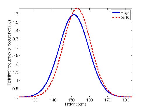
Sample distributions of the heights of boys and girls in the United States between 12 and 12.5 years of age. The plot shows the relative frequency of occurrence in percent with which the heights specified on the horizontal axis are observed.
Scientists describe these data with the same statistical tools used to help interpret measurement errors, that is, the average or mean values and the standard deviations:
| Mean Height (cm) |
Standard Deviation (cm) |
Sample Size |
|
| Boys | 151.43 | 8.05 | 573 |
| Girls | 153.19 | 7.48 | 576 |
In these samples, the average height of girls is slighter greater than the average height of boys. There is a great deal of overlap between the two distributions, however. Since all children are not being measured, the statistical uncertainty in the estimates of the mean heights must also be calculated in order to determine whether the mean heights are really different or whether the observed difference might simply have happened by chance.
The mean value computed from a specific set of measurements is only an estimate of the “true” mean. Scientists want to know the statistical uncertainty of this estimate. The uncertainty in the estimate of the mean value is just the standard deviation of the measurements (σ) divided by the square root of the number of measurements (n). The standard deviation of the mean, which is written σm, is:
$latex \displaystyle \sigma_{m} = \frac {\sigma}{\sqrt{n}} &s=3$
The standard deviations of the estimates of the mean heights are:
$latex \displaystyle \sigma_{m}{\scriptstyle(boys)} = \frac{8.05}{\sqrt{573}} = 0.34cm &s=3$
$latex \displaystyle \sigma_{m}{\scriptstyle(girls)} = \frac{7.48}{\sqrt{576}} = 0.31cm &s=3$
The difference in the mean heights is 1.76 cm (153.19 – 151.43), which is much greater than the standard deviations of the means. This suggests that the difference in the average heights of 12-year-old girls and boys is real and not due to chance. Scientists have developed a statistic called the t-test that compares the sample means with the standard deviations of the means to determine whether the two samples are different (see, for example, Trochim, W. M., “Research Methods Knowledge Base”). The t-test also allows scientists to determine the statistical level of significance. It is commonly accepted that the difference is statistically significant if there is only a 1 in 20 (5%) probability that the difference could be due to chance.
Given the large overlap between the two distributions in this case, rather large sample sizes are needed to have small enough standard deviations of the means to draw statistically significant conclusions. Not all situations are like this one, however. The following figure compares this case to two hypothetical cases with the same mean values, but with medium and low variability.
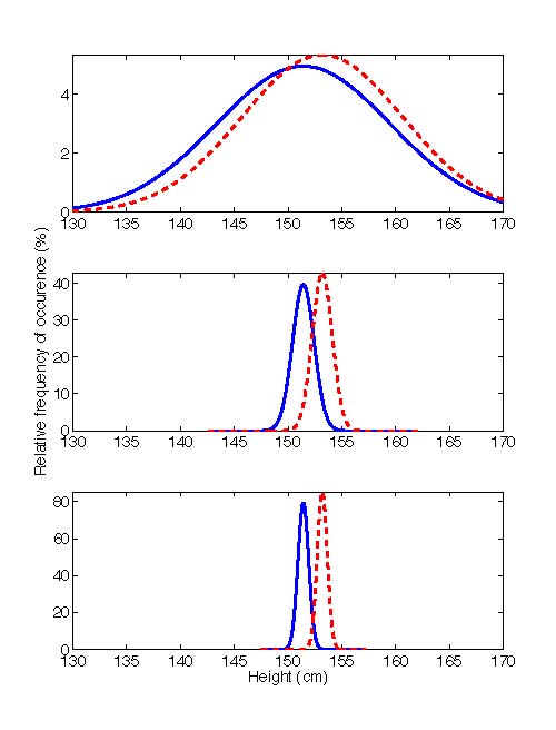
Sample distributions of the heights of boys and girls in the United States between 12 and 12.5 years of age (top), together with distributions with the same means as the actual sample distributions, but with standard deviations that are one-eighth (middle) and one-sixteenth (bottom) of the observed standard deviations.
In these graphs, the difference between the mean heights for boys and girls is the same in all three cases. However, because of the different levels of variability in the three cases, they look quite different. In the bottom, or low-variability case, the heights of boys and girls appear most dissimilar. In this case, there is the least overlap between the two groups, making it relatively easy to determine that the means are really different, even with only a limited number of samples. By comparison, in the top, or high-variability case, the heights of boys and girls appear most similar. Because the two distributions overlap so much in this case, much larger sample sizes are needed to determine whether the means are really different. In the low variability case, because the standard deviation is 16 times smaller than in the high variability case, a sample size (n) 1/16th as large would give the same standard deviation of the mean. The middle, or medium-variability case, is somewhere in between. It is important to consider the variability in the data when trying to determine from a set of measurements whether or not the means are really different.
Additional pages under Statistical Uncertainty:
- Measurement Errors are due to the physical limitations of the sensors and techniques used to make the measurements.
- False Positives and False Negatives are errors associated with making a decision.
- Statistical versus Biological Significance compares the results of statistical analyses within the range of natural variability.
Additional Resources
- Zales, C. R., and Colosi, J. C. 1998, “An Exercise Where Students Demonstrate the Meaning of ‘Not Statistically Significantly Different'” The American Biology Teacher. 60 (8), 596–600.
References
- Kuczmarski, R. J., Ogden, C. L., & Guo, S. . (n.d.). 2000 CDC growth charts for the United States: Methods and development (Vital Health Statistics No. 11) (p. 246). National Center for Health Statistics. Retrieved from https://www.cdc.gov/nchs/data/series/sr_11/sr11_246.pdf
- Trochim, W. M. (n.d.). The Research Methods Knowledge Base, 2nd Edition. Retrieved from https://conjointly.com/kb/