How is sound used to measure temperature in the ocean?
The speed of sound in water depends on the water properties of temperature, salinity and pressure (directly related to the depth). A typical speed of sound in water near the ocean surface is about 1520 meters per second. That is more than 4 times faster than the speed of sound in air. The speed of sound in water increases with increasing water temperature, increasing salinity and increasing depth. Most of the change in sound speed in the surface ocean is due to changes in temperature. This is because the effect of salinity on sound speed is small and salinity changes in the open ocean are small. Near shore and in estuaries, where the salinity varies greatly, salinity can have a more significant effect on the speed of sound in water. As the depth increases, the pressure of the water has the largest effect on the speed of sound.
The approximate change in the speed of sound with a change in each property:
Temperature 1°C = 4.0 m/s
Salinity 1PSU = 1.4 m/s
Depth (pressure) 1km = 17 m/s
Note: Changes in the speed of sound for a given property are not linear.
Under most conditions the speed of sound in water is simple to understand. Sound will travel faster in warmer water and slower in colder water. To measure the temperature of the water, a sound pulse is sent out from an underwater sound source and heard by a hydrophone in the water some distance away (up to thousands of kilometers). The time the sound takes to go from the source of the sound to the listening device (a hydrophone) is measured. From the travel time, the speed of sound between the source and the hydrophone can be calculated. If the salinity and depth where the sound traveled are known, the temperature of the water can be calculated. Two specific methods of measuring the temperature of the ocean with sound are explained below.

Schematic of an ocean acoustic tomography experiment. Black dots (S) are sound sources; open dots (R) are receivers (hydrophones). The dark area represents an ocean eddy with a different average sound speed than the surrounding ocean water.
Acoustic Tomography uses precise measurements of acoustic travel times to draw ocean temperature maps, showing ocean temperatures just as weather maps show temperatures in the atmosphere. Data from many crossing acoustic paths are used to generate these maps of ocean temperatures. In the figure above, for example, four acoustic sources (S) are shown transmitting to five acoustic receivers (R), giving 20 acoustic paths through a region roughly 300 kilometers on a side. (This geometry was actually used in an experiment conducted in 1981.) Suppose that the shaded region is warmer than its surroundings. Sound that travels through the warm region will travel slightly faster than sound that does not, because sound speed increases with increasing temperature, as described above. The travel times of sound pulses traveling through the warm region will therefore be slightly shorter than they would have been if the warm region was not there. By combining all of the different travel times it is possible to draw a map showing the warm and cold regions through which the sound has traveled. This is important because the ocean has “weather” just as the atmosphere does. Warm and cold “eddies” that are the oceanic equivalent of atmospheric storms move around, grow, and weaken. There are subsurface oceanic cold and warm fronts just as there are cold and warm fronts in the atmosphere. These eddies and subsurface fronts have important effects on marine life, with marine animals that prefer warm water tending to remain in warm eddies, for example.
The basic principles used in Acoustic Tomography are closely related to those used in CAT (Computed Axial Tomography) scans in medicine. In a CAT scan, the absorption of X-rays are used to map a “slice” through the human body. (“Tomo” is derived from the Greek word for cut or slice.) In Acoustic Tomography, the travel time of sound waves are used to map temperatures in a “slice” of the ocean.
Even when it is not feasible to have enough sources and receivers to make detailed temperature maps, acoustic travel times can be used to obtain the average temperatures along the paths which the sound traveled. This is sometimes called “acoustic thermometry.” The ATOC (Acoustic Thermometry of Ocean Climate) project measured average temperatures in the North Pacific Ocean, for example, along a number of paths. Acoustic sources off central California and north of Kauai (Hawaii) transmitted to U. S. Navy receivers, giving a sparse network of acoustic paths. They observed large-scale seasonal changes in ocean temperature. Transmissions continuing for many years could be used to measure large-scale climate change in the ocean.
Inverted Echosounders

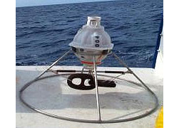
Inverted echo sounder. Photo courtesy of Dr. Randy Watts, URI/GSO
Inverted Echosounders (IES) measure the temperature of the water column at a single point. The IES is attached to the ocean bottom. It emits a sound pulse aimed toward the surface of the ocean. The sound pulse will reflect off the surface of the ocean and return to the bottom. The IES listens for the return of the sound pulse from the ocean surface. The travel time of the sound is used to calculate the speed of sound through the water. The temperature profile is calculated from the speed of sound through the water. The IES must be calibrated with a measurement of the water column properties. Sometimes a pressure sensor is used with the IES to make the calibration.
Inverted echosounders are often used to monitor a particular region of the ocean. They are often placed in groups (or arrays) to cover a wider area.
Animation of an inverted echo sounder.
Table of the speed of sound calculated under different ocean conditions.
Calculated using the simplified formula from Collins, 1981.
| Temperature (°C) | Salinity (S) | Depth (km) | Speed of Sound (m/s) | ||||
| 0 | 0 | 0 | 1402 | ||||
| 0 | 35 | 0 | 1449 | ||||
| 5 | 35 | 0 | 1470 | ||||
| 5 | 35 | 0 | 1470 | ||||
| 10 | 35 | 0 | 1490 | ||||
| 5 | 35 | 0 | 1470 | ||||
| 20 | 35 | 0 | 1521 | ||||
| 30 | 35 | 0 | 1545 | ||||
| 5 | 35 | 0 | 1470 | ||||
| 20 | 5 | 0 | 1488 | ||||
| 5 | 35 | 0 | 1470 | ||||
| 20 | 10 | 0 | 1493 | ||||
| 20 | 20 | 0 | 1505 | ||||
| 20 | 35 | 0 | 1521 | ||||
| 5 | 35 | 1 | 1487 | ||||
| 5 | 35 | 2 | 1503 | ||||
| 5 | 35 | 3 | 1521 | ||||
| 5 | 35 | 4 | 1539 |
Note: Changes in the speed of sound for a given property are not linear.
Additional Resources
- Able Sea Chicks Blog.
- Acoustic Thermometry of Ocean Climate (ATOC)
- ATOC Project Homepage.
- Spindel, R.C., and P.F. Worcester 1990, “Ocean acoustic tomography.” Scientific American, 263, 94-99 (October, 1990)
- National Academy of Sciences, Sounding Out the Oceans Secrets.
- URI-GSO IES Group.