How is sound used to measure global climate change?
Introduction
The average temperature of the ocean is rising as the global climate warms. Where the warming occurs and the rate at which it occurs are of great interest to climatologists. There are several difficulties in measuring the kinds of temperature changes that interest climatologists:
- Because the ocean is very large, it is difficult to get a complete picture of its temperature, and multiple measurements are required.
- The ocean is filled with warm and cold eddies, similar to storms in the atmosphere. The temperature changes associated with these eddies are large compared to the small, long-term changes in ocean temperature expected from climate change. Temperatures must be averaged over a wide area in order to identify a climate change signal.
- The temperature measurements must occur as frequently as possible over a long time period, in order to average out seasonal fluctuations and other short-term effects.
- Measurements must be taken throughout the water column.
Deploying sensors from ships will not provide sufficient temperature data. Although very accurate, many measurements must be collected frequently, over an extensive area to provide the large-scale averages needed. There are simply not enough ships to meet these requirements.
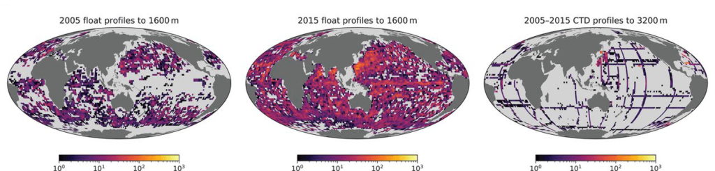
Approaches that provide more extensive data use drifting floats and satellite measurements of sea surface height. Drifting floats periodically descend to depths of 2000 m and then surface to send data back by satellite (https://argo.ucsd.edu). Data from thousands of floats are averaged to provide much of what scientists know about large-scale changes in ocean temperature since 2000. Satellite measurements of sea surface temperature provide global coverage at the surface of the ocean.
Acoustic Tomography
Another approach to measuring ocean temperatures is based on how sound speed varies. The speed of sound in water depends on pressure, temperature, and salinity. As any of these factors increase, sound speed also increases. Generally, temporal changes in ocean sound speed are dominated by temperature. By measuring the travel time of sound between two points, the average temperature of the water between the points can be calculated. Very precise measurements of the average temperature can be made with sound.

Acoustic tomography can be used to measure the temperature of the ocean over large areas. An acoustic source sends signals at precise times. Acoustic tomography sound sources are typically placed in the SOFAR channel to allow the sound to travel as far as possible. These low frequency tomography signals can travel thousands of kilometers in the ocean. Hydrophones deployed throughout the ocean are used to detect the signals. The signal travel time from the source to each hydrophone is used to calculate the average temperature along the path between the source and the receiver. The more sources and receivers that are deployed, the better spatial resolution of the temperature maps.
The travel time between a source and a hydrophone separated by about 5000 kilometers (3100 miles) takes approximately one hour. Over this range, the travel times can be measured to within 20-30 milliseconds. This travel time accuracy enables the determination of the average temperature to within a few millidegrees (thousandths of a degree) Celsius.
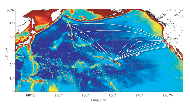
The first large scale demonstration of acoustic tomography was the Acoustic Thermometry of Ocean Climate (ATOC) project, which measured average temperatures in the North Pacific Ocean along a number of paths from 1996 to 2006. Acoustic sources deployed off central California and north of Kauai, Hawaii, transmitted signals to U. S. Navy receivers, creating a network of acoustic paths. This test verified that transmissions broadcast over many years could be used to measure long term changes in ocean temperature, possibly related to climate change.
Sources used in the ATOC project typically sent a signal for 20 minutes every 4 hours, every 4 days, resulting in 2 hours of signal transmission every 4 days. The source signals had a frequency range of 57-92 Hz, centered on 75 Hz with a bandwidth of 35 Hz. Low frequencies were used because they travel farther across the ocean than high frequencies. The signals were designed to minimize transmitted power (See the DOSITS page: Signal Processing).
The application of acoustic methods to study climate variability is especially compelling in ice-covered regions, where long-term, large-scale, continuous observations of the ocean interior have been difficult to obtain using other approaches. For example, gliders, profiling floats, and autonomous underwater vehicles that measure ocean temperature, salinity, and other variables cannot surface in ice-covered regions to use the Global Navigation Satellite System and relay data back to shore. Satellite measurements cannot be used to measure sea surface height in ice-covered areas. Acoustic tomographic systems, however, can operate beneath the ice to measure large-scale ocean temperature.
Seismic Ocean Thermometry
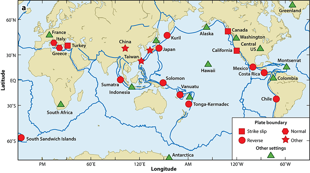
Seismic ocean thermometry uses naturally occurring earthquakes as a sound source to measure changes in ocean temperature. The first results using this method were reported in 2020 for a region of the Indian Ocean over a twelve-year span, 2004 to 2016. Most earthquakes cannot be used as a sound source for ocean thermometry, because their location cannot be determined with enough precision. However, a small subset of the world’s earthquakes are generated repeatedly from the exact same location along the same earthquake fault. They can repeat over a range of time scales; relatively short timescales, days to months, to longer time scales of decades and longer. Earthquakes generated from the same location can be recognized because they have nearly identical signal waveforms, and so two earthquakes generated years apart can be recognized as arriving from the same source by observing a high correlation in their signals. The key to seismic ocean thermometry is the use of these repeating earthquakes as the sound source. These types of earthquakes generally occur close enough to each other that any changes in travel time of a signal traveling from the earthquake location to receiver hundreds of kilometers away are dominated by changes in ocean sound speed, and not from the slight differences in earthquake location.
Earthquakes release large amounts of energy that propagate as seismic waves in the Earth. Seismic energy from earthquakes is converted into acoustic energy, t-waves, at the seafloor-water boundary. The acoustic energy from earthquakes is much greater than any anthropogenic sound source. T-waves have frequencies in the 1 Hz to 50 Hz range and can propagate long distances in the ocean. They are converted back to seismic waves when they encounter land and are recorded by near shore land-based seismometers (see How is sound used to study undersea earthquakes? for more information).
The seismic ocean thermometry results from the Indian Ocean show the same seasonal and annual variation as other temperature anomaly records of the region. In addition, the new record shows a decadal warming trend in ocean temperature, also similar to other temperature anomaly records. When there is sufficient data, as in 2005 and early 2006 in the Indian Ocean study, seismic ocean thermometry can record variation on the scale of days and weeks which is not usually possible with other methods.
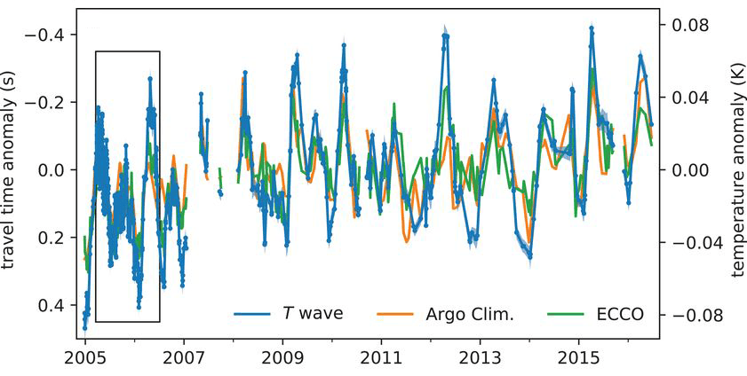
The magnitude of seasonal changes and the long-term increase in warming are larger for the seismic ocean thermometry results than the other records. The seismic ocean thermometry results illustrated above only used t-wave frequencies from 1.5 Hz to 2.5 Hz, which are sensitive to ocean temperature from the surface to the seafloor. In contrast, the current generation of Argo floats typically measure down to 2,000 m. Some variation between methods could be a result of the different effective depth ranges of the ocean that are sampled.
One limitation of seismic ocean thermometry is the timing and location of the acoustic signals. They are completely dependent on how often and where repeating earthquakes occur. This can lead to gaps in the record, as seen in the figure above in 2007 for example. Another limitation is using seismometers on land. This effectively limits the data to earthquakes above magnitude M4. However, using hydrophones to directly measure the sound in the ocean from earthquakes can expand the usable earthquakes to those below magnitude M4, perhaps as low as magnitude M1.8 (See How is sound used to study undersea earthquakes? for more information).
Future Measurements
Seismic ocean thermometry has great promise to expand the record of ocean temperature measurements. The demonstration of this method used archived records from three land-based seismometers to calculate the ocean temperature. There is a wealth of archived seismic data from earthquakes recorded at hundreds of seismometer locations that goes back decades in many cases. There are more than 10,000 shallow earthquakes of magnitude M4 or greater each year, so the data set will continuously grow.
Archived recordings from hydrophones, such as those used for the Comprehensive Nuclear-Test-Ban Treaty (CTBT), may be another source of data for seismic ocean thermometry. Drifting buoys with hydrophones onboard to collect earthquake t-wave data have been used to study the geology in specific regions of the ocean. A broader deployment of hydrophone equipped drifting buoys, such as the Argo floats, could further expand the volume of data and reduce gaps in the data leading to more robust temperature measurements.
DOSITS Links
- People > Research Ocean Physics > How is sound used to measure temperature in the ocean?
- People > Examine the Earth > How is sound used to study undersea earthquakes?
- People > Examine the Earth > How is sound used to study underwater volcanoes?
- People > National Defense > How is sound used to monitor nuclear testing?
- Science > How does sound travel long distances? The SOFAR Channel
- Technology Gallery > Hydrophone/Receiver
- Technology Gallery > Acoustic Tomographic Mooring
- Technology Gallery > CTBT Hydrophone Station
Additional Resources
- ARGO array (drifting buoys)
- EOS – Earthquakes reveal how quickly the Earth is warming
- Ars Techinca – Seismic sound waves crossing the deep ocean could be a new thermometer
- Acoustics Today Article – Ocean acoustics in the rapidly changing arctic
References
- Baringer, M., Bif, M. B., Boyer, T., Bushinsky, S. M., Carter, B. R., Cetinić, I., Chambers, D. P., Cheng, L., Chiba, S., Dai, M., Domingues, C. M., Dong, S., Fassbender, A. J., Feely, R. A., Frajka-Williams, E., Franz, B. A., Gilson, J., Goni, G., Hamlington, B. D., … Zhang, H.-M. (2020). Global Oceans. Bulletin of the American Meteorological Society, 101(8), S129–S184. https://doi.org/10.1175/BAMS-D-20-0105.1
- Dushaw, B. D., Worcester, P. F., Munk, W. H., Spindel, R. C., Mercer, J. A., Howe, B. M., Metzger, K., Birdsall, T. G., Andrew, R. K., Dzieciuch, M. A., Cornuelle, B. D., & Menemenlis, D. (2009). A decade of acoustic thermometry in the North Pacific Ocean. Journal of Geophysical Research, 114(C7), C07021. https://doi.org/10.1029/2008JC005124
- Dushaw, B. (2010). A Global Ocean Acoustic Observing Network. Proceedings of OceanObs’09: Sustained Ocean Observations and Information for Society, 259–271. https://doi.org/10.5270/OceanObs09.cwp.25
- Howe, B. M., Miksis-Olds, J., Rehm, E., Sagen, H., Worcester, P. F., & Haralabus, G. (2019). Observing the Oceans Acoustically. Frontiers in Marine Science, 6, 426. https://doi.org/10.3389/fmars.2019.00426
- Mikhalevsky, P. N., Sagen, H., Worcester, P. F., Baggeroer, A. B., Orcutt, J., Moore, S. E., Lee, C. M., Vigness-Raposa, K. J., Freitag, L., Arrott, M., Atakan, K., Beszczynska-Möller, A., Duda, T. F., Dushaw, B. D., Gascard, J. C., Gavrilov, A. N., Keers, H., Morozov, A. K., Munk, W. H., … Yuen, M. Y. (2015). Multipurpose Acoustic Networks in the Integrated Arctic Ocean Observing System. ARCTIC, 68(5), 11. https://doi.org/10.14430/arctic4449
- Nolet, G., Hello, Y., Lee, S. van der, Bonnieux, S., Ruiz, M. C., Pazmino, N. A., Deschamps, A., Regnier, M. M., Font, Y., Chen, Y. J., & Simons, F. J. (2019). Imaging the Galápagos mantle plume with an unconventional application of floating seismometers. Scientific Reports, 9(1), 1326. https://doi.org/10.1038/s41598-018-36835-w
- Okal, E. A. (2008). The generation of T waves by earthquakes. In Advances in Geophysics (Vol. 49, pp. 1–65). Elsevier. https://doi.org/10.1016/S0065-2687(07)49001-X
- Slack, P. D., Fox, C. G., & Dziak, R. P. (1999). P wave detection thresholds, Pn velocity estimates, and T wave location uncertainty from oceanic hydrophones. Journal of Geophysical Research: Solid Earth, 104(B6), 13061–13072. https://doi.org/10.1029/1999JB900112
- Spindel, R. C., & Worcester, P. F. (1990). Ocean acoustic tomography. Scientific American, 263, 94–99.
- Uchida, N. (2019). Detection of repeating earthquakes and their application in characterizing slow fault slip. Progress in Earth and Planetary Science, 6(1), 40. https://doi.org/10.1186/s40645-019-0284-z
- Uchida, N., & Bürgmann, R. (2019). Repeating Earthquakes. Annual Review of Earth and Planetary Sciences, 47(1), 305–332. https://doi.org/10.1146/annurev-earth-053018-060119
- Worcester, P. F., & Ballard, M. S. (2020). Ocean acoustics in the changing Arctic. Physics Today, 73(12), 44–49. https://doi.org/10.1063/PT.3.4635
- Worcester, P. F., Dzieciuch, M. A., & Sagen, H. (2020). Ocean acoustics in the rapidly changing arctic. Acoustics Today, 16(1). https://doi.org/10.1121/AT.2020.16.1.55
- Wu, W., Zhan, Z., Peng, S., Ni, S., & Callies, J. (2020). Seismic ocean thermometry. Science, 369(6510), 1510–1515. https://doi.org/10.1126/science.abb9519
- Wunsch, C. (2020). Advance in global ocean acoustics. Science, 369(6510), 1433–1434. https://doi.org/10.1126/science.abe0960