Ocean Noise Variability and Noise Budgets
Ocean Noise Variability
Sound levels in the ocean are not constant, but differ from location to location and change with time. Different sources of sound contribute to the overall noise level, including shipping, breaking waves, marine life, and other anthropogenic and natural sounds.
At low frequencies (20–500 Hz), the background sound level is dominated by noise from distant ships in many places in the ocean, even when there is no nearby ship. When a large ship passes close to a receiver, the noise that is generated will temporarily increase the sound levels at that location substantially. This is particularly true in areas of heavy shipping traffic, such as the area off the New England coast shown below.

Red and black lines are large commercial ship tracks from April and May 2006, respectively, off the northeast coast of the United States. Vessels are tracked using the U.S. Coast Guard’s Automatic Identification System. (Reprinted [with modifications] from Hatch et al., 2008.)

Spectrogram from a receiver on the continental slope off Point Sur, California, from January 1995 to January 2001,using 1-day averages. The increase in ambient noise at 17–20 Hertz during the fall and winter is due to blue and fin whale calls. (Reprinted with permission from Andrew et al. 2002.)
In the frequency range 500-100,000 Hz, ambient noise is mostly due to spray and bubbles associated with breaking waves. It increases with increasing wind speed. A storm passing over a receiver can temporarily increase mid-frequency sound level by 30 underwater dB or more, depending on the strength of the storm.

The appearance of the sea when the wind is at Force 10 as defined by the Beaufort Scale, corresponding to a wind speed of 48–55 knots. The wave height is 9–12.5 m (29–41 ft). (Reprinted from Bowditch, 1995).
Heavy rain associated with a storm can increase noise levels by up to 35 underwater dB across a broad range of frequencies extending from several hundred hertz to greater than 20,000 Hz.
One way to characterize the variability in underwater sound levels at specific locations is to make plots showing how often various sound levels occur. In these plots, a relative frequency of 0.1 means that sound level was observed 10% of the time.

Histograms showing the distribution of sound levels (dB re 1 µPa2 / Hz) at 50 Hz and 400 Hz as observed at a receiver on the continental slope off Pt. Sur, California, from November 1994 to December 2000. Each bin in the histogram is one dB wide. (Courtesy R. Andrew, Applied Physics Laboratory, University of Washington.
The plots above show that the sound levels at 50 Hz, where shipping noise dominates, are typically much higher than the sound levels at 400 Hz, where shipping noise is less important and noise from breaking waves is becoming more important. The differences between these sound level distributions can be partially described by their means, medians, and standard deviations, as shown below for the Pt. Sur data.
| Frequency (Hz) |
Mean (dB re 1 µPa2 / Hz) |
Median (dB re 1 µPa2 / Hz) |
Standard Deviation (dB re 1 µPa2 / Hz) |
| 50 | 91.3 | 90.6 | 4.8 |
| 100 | 81.0 | 80.2 | 4.9 |
| 200 | 75.7 | 75.2 | 4.4 |
| 400 | 71.6 | 71.1 | 4.0 |
The mean sound level is the average sound level. The median sound level is the level for which half of the observed sound levels are greater and half are smaller. The standard deviation is a measure of the width of the distribution about the mean. Approximately 68% of the observed sound levels are within one standard deviation of the mean, although the precise percentage depends on the shape of the distribution. At 50 Hz, for example, approximately 68% of the observations at Pt. Sur fall between 85.8 and 95.4 dB re 1 µPa2 / Hz.
Note that the observed distributions in the figures above are not symmetric, but rather tend to have “tails” extending toward higher sound levels. The average values (means) are therefore slightly greater than the medians. If the distributions were symmetric, the means and medians would be the same. At these relatively low frequencies, the occurrences of high sound levels are likely due at least in part to ships passing close to the receiver. It is important to take account of the distribution of observed sound values when assessing the potential importance of the ocean noise to marine life.
Ocean Noise Budgets
In addition to characterizing the variability in underwater sound levels by how often they occur, one can also characterize the relative contributions of different sources of underwater sound to the overall noise levels. At a frequency of 500 Hz, for example, shipping, wind (breaking waves), and rain all contribute to underwater sound levels. Over the course of a day, a receiver will therefore record changing sound levels as the contributions from all three sources vary.
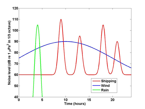
An example of possible contributions to sound levels at a receiver from shipping, wind, and rain at 500 Hz in a 1/3-octave frequency band over a day. Courtesy J. Miller, University of Rhode Island.
A noise budget is a listing of the various sources of noise at a receiver and their associated ranking by importance. It compares different sources of underwater sound, at particular geographical locations and in different frequency bands, averaged over time. A noise budget characterizes the magnitude of sound intensity or energy in the underwater sound field from various sources.
Ambient noise measurements made in the Ionian Sea, near Greece, with Passive Acoustic Listeners (PALs) have been used to determine the noise budget in 1/3-octave bands for this location. Ambient noise levels are often characterized by giving the noise level in 1/3-octave bandwidths. An octave is the interval between two frequencies when the higher frequency is twice the lower frequency. The center frequencies of the octave bands used in acoustics are usually chosen to be:
31.5 Hz, 63 Hz, 125 Hz, 250 Hz, 500 Hz, 1 kHz, 2 kHz, 4 kHz, 8 kHz, and 16 kHz
Each octave band is in turn split into three bands to give 1/3-octave bandwidths, providing a more detailed description of the frequency content of the noise.

The noise budget for the Ionian Sea during the period from 10 January 2004 to 17 April 2004 in a 1/3-octave bandwidth centered at 500 Hz. Reprinted [with modifications] from Miller et al., 2008.
Summary
Noise distributions and noise budgets are used in marine mammal masking studies (see What are the anthropogenic effects of sound on marine mammals? Masking), habitat characterization, and environmental studies. They are also used when designing acoustic communication and sonar systems.
Additional Links on DOSITS
- How is sound used to measure the upper ocean?
- How is sound used to measure waves in the surf zone?
- Rainfall
- Ship
Additional Resources
- Hatch, L. T., & Wright, A. J. (2007). A Brief Review of Anthropogenic Sound in the Oceans. International Journal of Comparative Psychology, 20, 121–133.
References
- Andrew, R. K., Howe, B. M., Mercer, J. A., & Dzieciuch, M. A. (2002). Ocean ambient sound: Comparing the 1960s with the 1990s for a receiver off the California coast. Acoustics Research Letters Online, 3(2), 65–70. https://doi.org/10.1121/1.1461915
- Bowditch, N. (1995). The American Practical Navigator. Bethesda, Maryland.: National Imagery and Mapping Agency.
- Hatch, L., Clark, C., Merrick, R., Van Parijs, S., Ponirakis, D., Schwehr, K., … Wiley, D. (2008). Characterizing the Relative Contributions of Large Vessels to Total Ocean Noise Fields: A Case Study Using the Gerry E. Studds Stellwagen Bank National Marine Sanctuary. Environmental Management, 42(5), 735–752. https://doi.org/10.1007/s00267-008-9169-4
- Miller, J. H., Nystuen, J. A., & Bradley, D. L. (2008). Ocean Noise Budgets. Bioacoustics, 17(1–3), 133–136. https://doi.org/10.1080/09524622.2008.9753791
- National Research Council (U.S.) (Ed.). (2003). Ocean noise and marine mammals. Washington, D.C: National Academies Press.
- Wenz, G. M. (1962). Acoustic ambient noise in the ocean: Spectra and sources. The Journal of the Acoustical Society of America, 34(12), 1936–1956. https://doi.org/10.1121/1.1909155