Measurement Errors
In order to understand the effects of measurement errors, consider the example of determining the speed of sound in seawater at a particular temperature, salinity, and pressure. This requires precise measurements of the distance between a sound source and receiver, the time that it takes the sound to travel from the source to receiver, and the temperature, salinity, and pressure of the seawater through which the sound travels. Although there is only one true value for the speed of sound at a given temperature, salinity, and pressure, two measurements will almost always yield different values of sound speed because of inaccuracies in the measurements. If the measurements are repeated many times, a range of values for the speed of sound at a specific temperature, salinity, and pressure will be obtained.
In early experiments to determine the speed of sound, such as that carried out by Colladon and Sturm in 1826, the measurements were not very accurate. The value that they reported for the speed of sound in Lake Geneva, Switzerland, at a temperature of 8°C was 1435 m/s, which is about 4 m/s slower than the modern value for fresh water at 8°C and atmospheric pressure (1439.07 m/s). If the measurement had been repeated 100 times, the measurement errors would have led to a range of values for the speed of sound, perhaps similar to the range shown in the histogram in the following figure. Each vertical bar in the figure gives the number of times that the measured sound speed falls within a 1 m/s range. The vertical bar centered at the value of 1435 m/s reported by Colladon and Sturm (arrow) shows that the measured value fell between 1434.5 and 1435.5 m/s seven times in this particular set of 100 simulated measurements, for example.
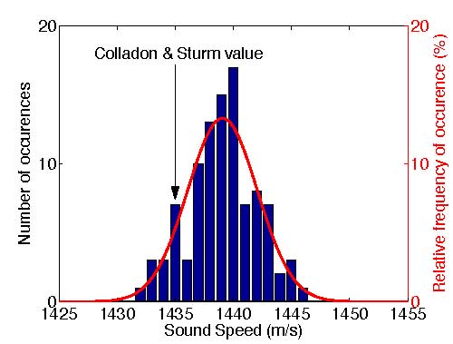
Histogram showing the number of times (left axis) that the measured sound speed might have fallen within 1 m/s intervals if the Colladon and Sturm experiment were repeated 100 times, constructed using a rough estimate of the uncertainties in their measurements. If the measurements were repeated many more times, the histogram would eventually approximate the smooth curve showing the relative frequency of occurrence in percent (right axis) with which the sound speeds specified on the horizontal axis would be observed for the uncertainties in the measurements assumed to construct the histogram.
The most basic statistic that scientists compute to help interpret multiple measurements is the average value of the measurements. In the example above, the average of 100 measurements provides a better estimate of the true sound speed than any single measurement. The average or mean (indicated by the symbol m) of a set of measurements is defined to be the sum of all of the measurements (indicated by the symbols x1, x2, … xn) divided by the number of measurements (indicated by the symbol n):
$latex m= \frac{(X_{1} + X_{2} + \ldots + X_{n})}{n} &s=2$
The mean value of the 100 measurements shown above is 1439.09 m/s, which is very close to the “true” value of 1439.07 m/s.
The next statistic that scientists compute to help interpret multiple measurements is a measure of the variability in the measurements. The standard deviation, which is usually indicated by the Greek letter σ (pronounced “sigma”) is a measure of the spread of the distribution about the mean. It is calculated by subtracting the mean from each of the measurements to obtain the differences between the measurements and the mean. One then computes the squares of the differences, adds all of the squared differences together, and divides by one less than the total number of measurements n. This calculation gives an estimate of the variance of the distribution when one has n measurements. The square root of the variance is the standard deviation:
$latex \sigma = \sqrt{ \frac{(X_{1} – m)^2 + (X_{2} – m)^2 + \ldots + (X_{n}-m)^2}{(n-1)}} &s=2$
The standard deviation of the 100 measurements shown above is 3.10 m/s. In this case, the standard deviation reflects an estimate of the uncertainty in Colladon and Sturm’s measurements that was used to construct the histogram.
The mean value computed from a specific set of measurements is only an estimate of the “true” mean. Scientists want to know the statistical uncertainty of this estimate. How accurate is the estimate of the sound speed in fresh water at 8°C and atmospheric pressure computed from the 100 measurements in the simulated example given above, for example? The uncertainty in the estimate of the mean value is just the standard deviation of the measurements (σ) divided by the square root of the number of measurements (n). The standard deviation of the mean, which is written σm, is:
$latex \displaystyle \sigma_{m} = \frac {\sigma}{\sqrt{n}} &s=3$
The standard deviation of the mean is often also called the standard error of the mean. For the case shown above, the standard deviation of the mean is:
$latex \displaystyle \sigma_{m} = \frac {3.10}{\sqrt{100}} = 0.31m/s &s=3$
The standard deviation of the mean specifies the statistical uncertainty of the estimate of the mean, due to the limited accuracy and precision of the measurements. This set of simulated measurements gives the value of sound speed in fresh water at 8°C and atmospheric pressure as 1439.09 ± 0.31 m/s. This means that the true value of the mean is likely to fall within a range of values 0.31 m/s above or below the calculated mean of 1439.09 m/s.
Modern experiments in which sound speed is measured in the laboratory are much more accurate than the experiment that Colladon and Sturm conducted in Lake Geneva, but the measurements are still not perfect. The modern “true” value is also uncertain and is most properly written as 1439.07 ± 0.05 m/s.
Additional pages under Statistical Uncertainty:
- Natural Variability is the range in values of naturally occurring parameters in biological and other natural systems.
- False Positives and False Negatives are errors associated with making a decision.
- Statistical versus Biological Significance compares the results of statistical analyses within the range of natural variability.
Additional Links on DOSITS
- How fast does sound travel?
- Scientific Method
- Scientific Uncertainty
- The First Studies of Underwater Acoustics: The 1800s\